A one-dimensional stochastic process

The theory

Take, for example, the well-documented one-dimension Ornstein—Uhlenbeck process, also known as Vašíček process. This process is governed by two main parameters: the mean-reverting parameter \(\theta\) and the diffusion or volatility coefficient \(\sigma\)

\[\mathrm{d}y(t) = -\theta y(t)\mathrm{d}t + \sigma \mathrm{d}W(t)\]

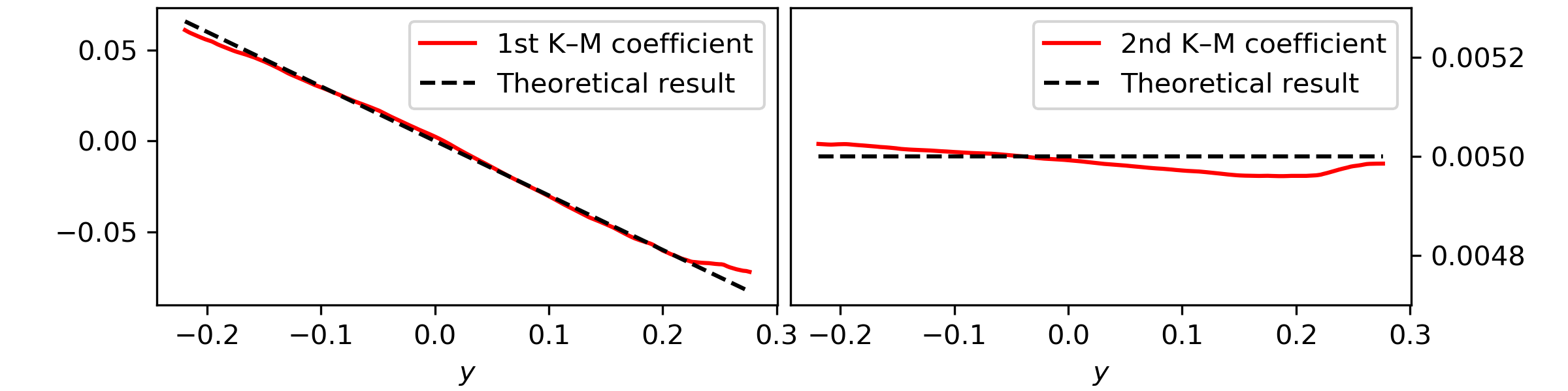
which can be solved in various ways. For our purposes, recall that the drift coefficient, i.e., the first-order Kramers—Moyal coefficient, is given by \(\mathcal{M}^{[1]}(y) = -\theta y\) and the second-order Kramers—Moyal coefficient is \(\mathcal{M}^{[2]}(y) = \sigma^2 / 2\), i.e., the diffusion.

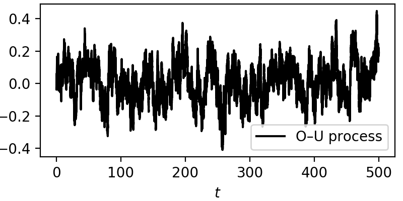
For this example let’s take \(\theta=0.3\) and \(\sigma=0.1\), over a total time of 500 units, with a sampling of 1000 Hertz, and from the generated data series retrieve the two parameters, the drift \(-\theta y(t)\) and diffusion \(\sigma\).

Integrating an Ornstein—Uhlenbeck process

Here is a short code on generating a Ornstein—Uhlenbeck stochastic trajectory with a simple Euler–Maruyama integration method

# integration time and time sampling
t_final = 500
delta_t = 0.001

# The parameters theta and sigma
theta = 0.3
sigma = 0.1

# The time array of the trajectory
time = np.arange(0, t_final, delta_t)

# Initialise the array y
y = np.zeros(time.size)

# Generate a Wiener process
dw = np.random.normal(loc = 0, scale = np.sqrt(delta_t), size = time.size)

# Integrate the process
for i in range(1,time.size):
    y[i] = y[i-1] - theta*y[i-1]*delta_t + sigma*dw[i]

From here we have a plain example of an Ornstein—Uhlenbeck process, always drifting back to zero, due to the mean-reverting drift \(-\theta y(t)\). The effect of the noise can be seen across the whole trajectory.

Using kramersmoyal

Take the timeseries \(y(t)\) and let’s study the Kramers—Moyal coefficients. For this let’s look at the drift and diffusion coefficients of the process, i.e., the first and second Kramers—Moyal coefficients, with an epanechnikov kernel

# Choose number of points of you target space
bins = np.array([5000])

# Choose powers to calculate
powers = np.array([[1], [2]])

# Choose your desired bandwith
bw = 0.15

# The kmc holds the results, where edges holds the binning space
kmc, edges = km(y, kernel = kernels.epanechnikov, bw = bw, bins = bins, powers = powers)

This results in

Notice here that to obtain the Kramers—Moyal coefficients you need to divide kmc by the timestep delta_t. This normalisation stems from the Taylor-like approximation, i.e., the Kramers—Moyal expansion (\(\delta t \to 0\)).