A two-dimensional diffusion process

Theory

A two-dimensional diffusion process is a stochastic process that comprises two \(W(t)\) and allows for a mixing of these noise terms across its two dimensions.

\[\begin{split}\begin{pmatrix} \mathrm{d}y_1(t) \\ \mathrm{d}y_2(t) \end{pmatrix}= \begin{pmatrix} N_1(y) \\ N_2(y) \end{pmatrix} \mathrm{d} t + \begin{pmatrix} g_{1,1}(y) & g_{1,2}(y) \\ g_{2,1}(y) & g_{2,2}(y) \end{pmatrix} \begin{pmatrix} \mathrm{d}W_1 \\ \mathrm{d}W_2 \end{pmatrix}\end{split}\]

with \(N\) the drift vector and \(g\) the diffusion matrix, which can be state dependent. We define, as the previous example, a process identical to the Ornstein—Uhlenbeck process, with

\[\begin{split}N = \begin{pmatrix} - N_1 y_1 \\ - N_2 y_2 \end{pmatrix}\end{split}\]

and we take \(N_1=2.0\) and \(N_2=1.0\). For this particular case a more involved diffusion matrix \(g\) will be used. Let the matrix \(g\) be state-dependent, i.e., dependent of the actual values of \(y_1\) and \(y_2\) via

\[\begin{split}g = \begin{pmatrix} \frac{g_{1,1} }{1+e^{y_1^2}} & g_{1,2} \\ g_{2,1} & \frac{g_{2,2} }{1+e^{y_2^2}} \end{pmatrix}\end{split}\]

and we will take \(g_{1,1} = g_{2,2}=0.5\) and \(g_{1,2} = g_{2,1} = 0\).

Integrating a 2-dimensional process

Taking the above parameters and writing again an Euler–Maruyama integration method

# integration time and time sampling
t_final = 2000
delta_t = 0.001

# Define the drift vector N
N = np.array([2.0, 1.0])

# Define the diffusion matrix g
g = np.array([[0.5, 0.0], [0.0, 0.5]])

# The time array of the trajectory
time = np.arange(0, t_final, delta_t)

# Initialise the array y
y = np.zeros([time.size, 2])

# Generate two Wiener processes with a scale of np.sqrt(delta_t)
dW = np.random.normal(loc = 0, scale = np.sqrt(delta_t), size = [time.size, 2])

# Integrate the process (takes about 20 secs)
for i in range(1, time.size):
    y[i,0] = y[i-1,0]  -  N[0] * y[i-1,0] * delta_t + g[0,0]/(1 + np.exp(y[i-1,0]**2)) * dW[i,0]  +  g[0,1] * dW[i,1]
    y[i,1] = y[i-1,1]  -  N[1] * y[i-1,1] * delta_t + g[1,0] * dW[i,0]  +  g[1,1]/(1 + np.exp(y[i-1,1]**2)) * dW[i,1]

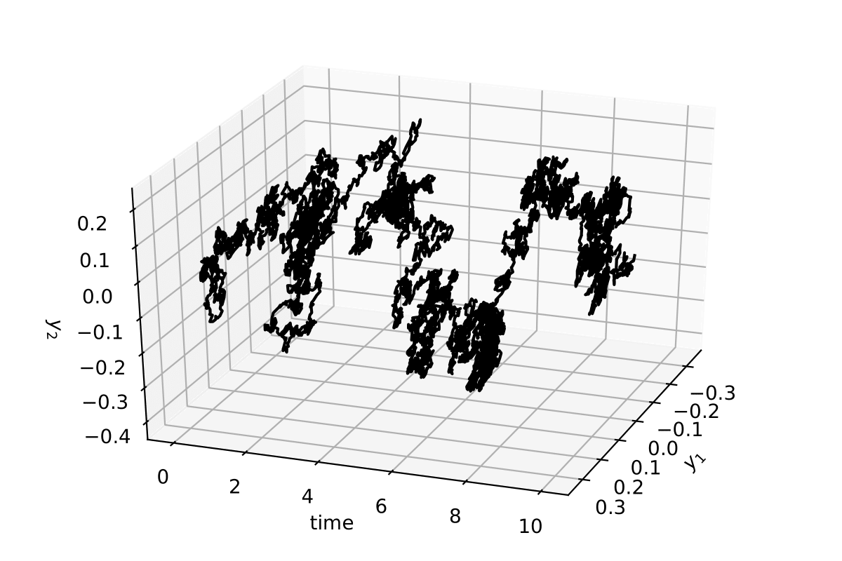
The stochastic trajectory in 2 dimensions for 10 time units (10000 data points)

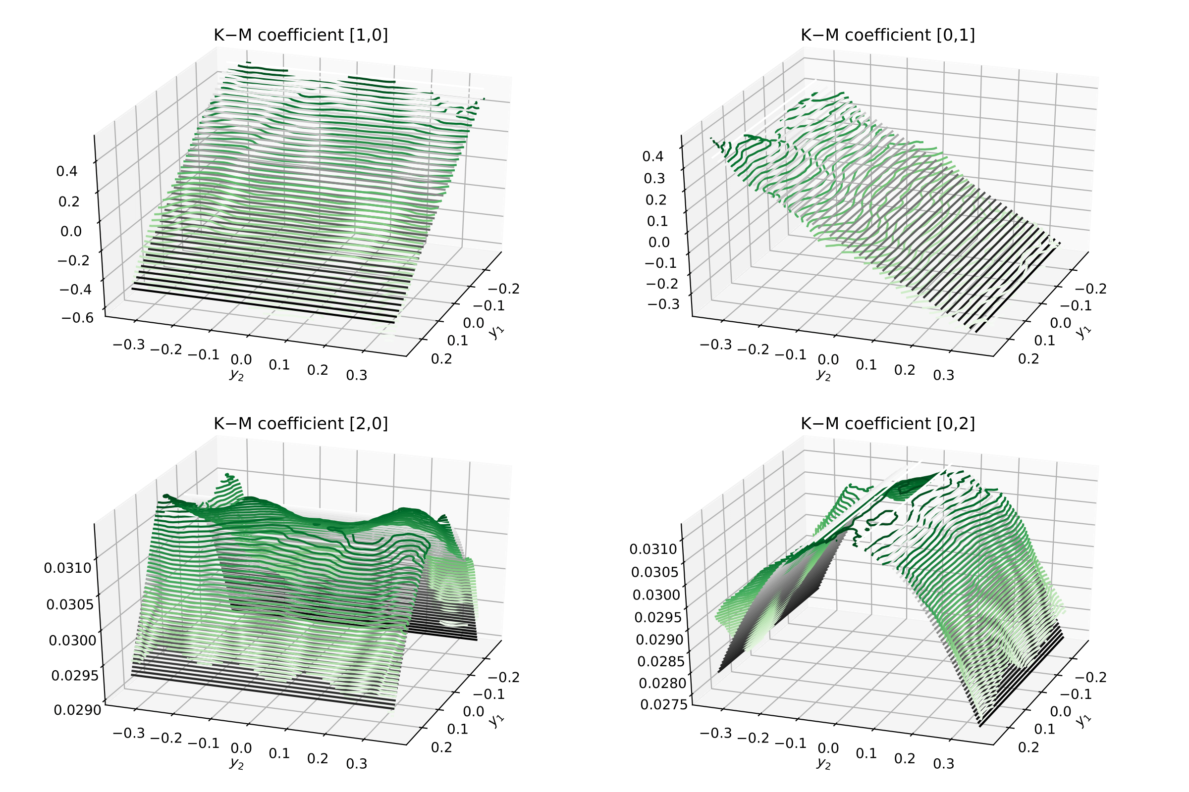
Back to kramersmoyal and the Kramers—Moyal coefficients

First notice that all the results now will be two-dimensional surfaces, so we will need to plot them as such

# Choose the size of your target space in two dimensions
bins = np.array([300, 300])

# Introduce the desired orders to calculate, but in 2 dimensions
powers = np.array([[0,0], [1,0], [0,1], [1,1], [2,0], [0,2], [2,2]])
# insert into kmc:   0      1      2      3      4      5      6

# Notice that the first entry in [,] is for the first dimension, the
# second for the second dimension...

# Choose a desired bandwidth bw
bw = 0.1

# Calculate the Kramers−Moyal coefficients
kmc, edges = km(y, bw = bw, bins = bins, powers = powers)

# The K−M coefficients are stacked along the first dim of the
# kmc array, so kmc[1,...] is the first K−M coefficient, kmc[2,...]
# is the second. These will be 2-dimensional matrices.

Now one can visualise the Kramers–Moyal coefficients (surfaces) in green and the respective theoretical surfaces in black. (Don’t forget to normalise: kmc / delta_t).